Approaches to RF Interference Suppression for VHF/UHF Synthetic Aperture Radar

Richard T. Lord and Michael R. Inggs

The authors are with the Radar Remote Sensing Group, University of Cape Town, Rondebosch 7701, South Africa. Phone +27 21 650 2799, Fax +27 21 650 3465, Email: rlord-avoidspam@ebe.uct.ac.za.

Note --- This paper has been published at the Comsig'98 conference. A pdf version of this paper can be downloaded here: comsig98a.pdf

Abstract --- An increasing amount of interest has developed in VHF/UHF SAR applications. Unfortunately the VHF-UHF portion of the spectrum is already in heavy use by other services, such as television and mobile communications. Even in remote locations the interference power often exceeds receiver noise by many dB, becoming the limiting factor on system sensitivity and severely degrading the image quality. This paper addresses the problem of radio frequency (RF) interference and its impact on SAR imagery. Several RF interference suppression methods are described and discussed. These include spectral estimation and coherent subtraction algorithms, as well as various filter approaches. The least-mean-squared (LMS) adaptive filter is described in detail, and its effectiveness in suppressing RF interference is demonstrated on simulated data and on real P-Band data.

Keywords --- Radio frequency interference, RFI, LMS adaptive filter, synthetic aperture radar, SAR, VHF, UHF.

1 Introduction

Ultrawideband radar has proven to be a very powerful method for underground and obscured object detection. The combination of using low frequencies (which exhibit very good foliage and ground penetrating capabilities) such as VHF/UHF or even lower, and using wideband pulses (which provide high range resolution), creates a wide variety of applications, making these radar systems extremely useful. Such applications include the detection of targets concealed by foliage and/or camouflage, detection of buried objects, detection and location of buried pipes and cables, and archaeological and geological exploration, such as the location of underground riverbeds. However these frequency bands are already in use by other services such as television, mobile communications, radio and cellular phones. The interference power received from these emitters often exceeds the receiver noise by many dB, thereby limiting the system sensitivity. Regulatory sanctions do not allow the increase of radar power, so that prior services are not appreciably degraded. Therefore it is important to investigate possible means of suppressing the interference in the received signal.

Suppressing radio interference from a received signal essentially involves three steps [1]:

Finding a model to parameterise the interfering signals,
estimating the parameters of the interfering signals using the measured data, and
using the estimated parameters to suppress the interference in the data.

Section 2 discusses the model which is commonly used to parameterise the interfering signals, and Section 3 gives a very brief literature review of approaches that have been used successfully to suppress RF interference. An approach that has received very favourable review is the least-mean-squared (LMS) adaptive filter [1, 10, 16]. It is described in detail in Section 4, and the results that have been obtained from simulated data and from real P-Band data are discussed in Section 5 and Section 6 respectively.

2 Modelling the RFI Environment

It is important to describe the interference environment as accurately as possible. This includes statistics on the density of the interference emitters, identity (type) of emitters, effective radiated power, modulation bandwidth, duty factor and temporal dependence. The most direct way to achieve this is to make use of ``sniffer'' pulses or ``listening beforehand'' schemes, however this is not yet generally implemented in practice. Although this method is useful for many signal processing methods, its effectiveness depends strongly on how long the RFI remains coherent.

Most approaches model the RFI as a superposition of single sinusoidal ``tones'', and the wideband signal plus system noise as white noise. Surveys performed by the Grumman E-2C UHF radar (420-450MHz) [9] have shown that 50% of emitters have a spectral bandwidth between 0-50kHz (single channel voice/radio telegraphy), 40% between 50-150kHz and less than 10% have a bandwidth greater than 150kHz (data communications, multichannel telephony, etc.)

It is important to estimate the modulation time of the RFI, which is the inverse of the RFI bandwidth, in order to predict whether the parameters of the modelled sinusoidal interference change across one range line, i.e. whether the tone model of the RFI breaks down. According to Braunstein et al [2], most RFI has a modulation time of 5-10 s, which is consistent with an effective bandwidth of a few hundred kHz or less.

3 Approaches to RFI Suppression

RFI suppression algorithms fall into two classes, namely (1) spectral estimation and coherent subtraction approaches and (2) various filter approaches. The relative merits and disadvantages of these approaches are discussed in the following subsections. One approach that has not been investigated is the creation of antenna pattern nulls in the direction of the RFI source as a means for suppressing the interference.

3.1 Spectral estimation and coherent subtraction approaches

These approaches have been shown to be extremely effective and powerful to the extent that the model of RFI as a superposition of sinusoids is true. They require the frequency, phase and amplitude

of each interfering sinusoid to be estimated, after which the sinusoids are subtracted from the contaminated signal. The performance is excellent in terms of low signal distortion and good interference suppression, however the effectiveness is reduced for high modulation bandwidths, since the parameters change over the record length. For computational efficiency and effectiveness, these methods must be ``tuned'' to use a priori knowledge, such as where the FM-broadcast band is located [13]. Furthermore the parameters of the tones (especially the phase) must be estimated for every pulse.

Braunstein et al [2] have achieved very good results using a maximum likelihood estimate (MLE) approach. For a single sinusoid in white noise the parameter vector can be found analytically, however for multiple sinusoids it becomes an extremely difficult nonlinear problem involving 3m variables, where m is the number of sinusoids to be estimated. An efficient technique to overcome this problem is to use an iterative algorithm, where the initial guess of the estimates is iteratively improved. The initial guess may be obtained from the data spectrum by applying an FFT. Another method would be to model the RFI, signal and noise as an autoregressive (AR) process [1, 12]. The estimate of the nth sample of the measured data is given by

equation90

where p is the order of the model, indicating that p/2 sinusoids can be estimated, a[k] are the autoregressive parameters which need to be derived from the measured data, and u[k] is the signal plus noise (without interference). According to Braunstein et al [2] the results obtained using this method are similar to those obtained using the MLE method.

Golden et al [7] used a parametric maximum likelihood (PML) algorithm for the estimation of the parameters of the RFI tones. This algorithm is also applied to deramp SAR. It is claimed that 90-95% of the RFI that could have corrupted a SAR image is removed. The number of iterations through the PML algorithm at each threshold is approximately equal to the number of tones being estimated.

Miller et al [13] have developed a chirp-least-squares algorithm with clipping (CLSC). The following advantages are claimed, compared to adaptive FIR filtering:

An estimate-and-subtract algorithm provides the narrowest possible stop-band for a given data length and therefore minimises time-sidelobes.
The CLSC technique allows iterative, nonlinear signal (target) excision, which reduces sidelobes and signal loss even further.
There are no filter edge effects.

This method makes use of a priori knowledge of the RFI environment. A non-least-squares approach is used to model FM signals, which vary by as much as 75kHz from the centre frequency.

Ferrell [5] has developed a method which requires 2-D compression of the SAR image (containing both signal and interference), after which a second compressed SAR image (containing only interference) is coherently subtracted. This requires two arrays of data to be collected in an interleaved manner, which might require the PRF to be increased by a factor of 2. It is claimed that this method leaves the target and clutter phase history essentially intact.

3.2 Filter approaches

A common suppression approach is to examine the spectrum of the contaminated signal, identify the interference spikes which are usually many dB larger than the signal, and then to remove these spikes with a notch filter. Although the notching concept is effective for very narrowband interferers and a small number of emitters, it can also produces adverse effects on the overall radar system performance [9], such as reducing image intensity, reducing range resolution, creating loss in the target's integrated signal to noise ratio and introducing time-sidelobes.

Koutsoudis and Lovas [9] describe an RFI Minimisation algorithm developed by Grumman Aerospace Corporation, which is based on least-mean-squared estimation theory. A single filter is used to achieve both the interference suppression as well as the equalisation needed to overcome the distortions caused by the notching function. This method has been tested extensively using numerous data sets and excellent performance results have been obtained for all scenarios.

Buckreuss [3] has implemented a notch filter to suppress RF interference in contaminated P-Band data. The interferences have been removed to a large extent, with some sidelobes visible in areas with intense backscatter, as well as a slight degradation of the contrast.

Abend and McCorkle [1] have achieved good results using an adaptive FIR filter approach. The adaptive filter is an over-determined system producing a FIR filter with n taps, independent of the number of interfering signals. As opposed to tone extraction methods, this method simultaneously eliminates hundreds of narrowband interferers. A low update rate for the filter tap weights is allowed, since the filter weights were found to be effective for hundreds of subsequent radar pulses. Furthermore, minimal computational complexity is required, making this a very fast method. An iterative technique has been used to reduce the range sidelobes caused by the filter's impulse response. The adaptive filter is based on an autoregressive (AR) all-pole interference model, which also models the RFI as sinusoidal tones. However the sinusoidal model only needs to be valid across the relatively short filter length. Furthermore the filter only depends on spectral energy, so the tap weights are not affected by the phase of the interference tone. A further advantage is that the adaptive filter ``learns'' the environment. It is claimed that the interference suppression filter can be superior to the tone extractor [1]. A disadvantage of using a filter approach is the reduction in record length because of edge effects.

Le et al [10] have implemented an LMS adaptive filter with very good results. The filter performance with respect to the filter parameters is analysed in terms of the radar performance parameters such as the integrated sidelobe ratio (ISLR) and peak sidelobe ratio (PSLR).

4 The LMS Adaptive Filter

Adaptive filters have been widely used in interference suppression applications [1, 6, 10, 11, 16]. In contrast to fixed filters, they have the desired ability to adjust their own parameters automatically. Little or no a priori knowledge of the signal or noise characteristics is required. It is, however, assumed that the interference is sinusoidal. The adaptive filter relies on a recursive algorithm, which, in a stationary environment, converges to the optimum Wiener solution. In a non-stationary environment, the algorithm offers a tracking capability, whereby it can track time variations in the statistics of the input data.

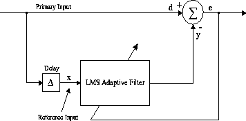Figure 1: LMS Adaptive Filter

Figure 1 shows a schematic of the LMS adaptive filter as it is used for RF interference cancelling. It requires a primary input d and a reference input x, which is obtained by delaying the primary input for some time delay . The adaptive linear combiner weighs and sums a set of input signals to form an adaptive output. The n-element input signal vector and the weight vector are defined at time j as follows:

and

The reference signal vector is defined as

The output y(j) of the filter is equal to the inner product of the row vectors and

This output is an estimate of the RF interference. The error signal e(j), which is the desired cleaned radar signal, is obtained by subtracting the RF interference estimate from the primary input d(j) according to

The LMS adaptive algorithm minimises the mean-square error e(j) by recursively altering the weight vector at each sampling instant according to the Widrow-Hoff algorithm [15], yielding

where the * symbol designates complex conjugation and is a convergence factor controlling stability and rate of adaptation. A larger value of increases the rate of convergence, but also leads to a larger final misadjustment, which is a quantitative measure of the amount by which the final value of the mean-squared error deviates from the minimum mean-squared error that is produced by the optimum Wiener filter.

5 Simulation Setup and Results

The adaptive filter was applied on simulated data to verify its suitability for RF interference suppression. Table 1 lists the relevant radar parameters of the simulation. These parameters correspond to the real P-Band data analysed in Section 6. The optimum filter parameters can then be used for suppressing the RF interference in the P-Band data.

Table 1: Radar Parameters of simulated and P-Band Data

centre frequency	450 MHz
chirp bandwidth	18 MHz
pulse length	5 s
A/D (complex) sample rate	60 MHz
range bins	2048

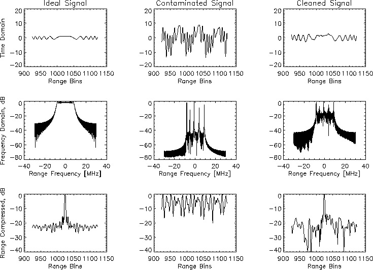
The simulation was assembled as follows: A clean signal (see first column of Figure 2) representing the ideal return of a single point target was injected with basebanded RF ``interference'' in the form of five pure sinusoids at frequencies -8, -5, -1, 4 and 9MHz with corresponding interference-to-signal amplitude ratios of 6, 2, 7, 4 and 5dB respectively and with random phase (see second column of Figure 2). White noise with a SNR of 20dB was also added. This contaminated signal was fed to the adaptive filter (see third column of Figure 2), and the performance of the filter was evaluated by range compressing the filter output and measuring the target mainlobe width, the peak sidelobe ratio (PSLR) and the integrated sidelobe ratio (ISLR), measured across 200 range bins.

Figure 2: Simulation results demonstrating the effectiveness of the adaptive filter applied to RF interference suppression. The three columns show the ideal, contaminated and cleaned signal respectively. The first row shows the real part of the signal in the time domain, the second row shows the signal in the frequency domain, and the third row shows the range compressed signal.

5.1 Filter Performance

Table 2 gives an indication of how the radar performance is affected by the number of filter weights and the convergence factor

. The delay

has not been included, since it was found that a delay of one time sample was sufficient, and larger values of

did not affect the results significantly. It has to be noted that the value of

is inversely dependent on the amplitude of the input vector, and therefore the absolute value is not as important as the relative change with respect to the number of weights. Furthermore, as the number of weights increases, the value of

needs to be decreased appropriately, otherwise the filter output becomes unstable. This can be seen in Table 2 with 256 weights and

. Generally the performance increases as

decreases. However if

becomes too small, the weights do not converge, which also yields poor performance. This was the case with 20 weights and

. The results also improve as more weights are used, however this increases computation time and edge effects.

**Table 2:** Radar Performance vs Filter Parameters
Filter Parameters		Radar Performance
weights		ML Width	PSLR	ISLR
		[range bins]	[dB]	[dB]
20	1e-4	3.1	-5.30	3.09
20	1e-5	3.2	-7.27	1.20
20	1e-6	3.4	-1.73	10.2
100	1e-4	2.9	-3.08	7.15
100	1e-5	3.1	-9.97	-0.68
100	1e-6	3.2	-12.4	-0.63
256	1e-4	unstable	unstable	unstable
256	1e-5	3.0	-7.89	0.40
256	1e-6	3.2	-12.9	-2.78

Figure 2 graphically illustrates the results that were obtained with 256 weights and

. The first column displays the ideal signal, without any interference. The second column displays the contaminated signal, with the spectrum completely dominated by noise and interference. The point target is not detectable in the range compressed signal shown in the last row. The third column shows the output of the adaptive filter, which is clearly a vast improvement compared to the noisy signal. Looking at the second row, the filter has significantly suppressed the spikes caused by the sinusoidal interferences. The point target is clearly visible in the range compressed signal, with the peak sidelobe being -12.9dB below the mainlobe, using a rectangular weighting window.

5.2 Performance Optimisation

The adaptive filter has been modified as follows in order to improve the performance measured in terms of the PSLR and ISLR:

The range compressed output of the adaptive filter sometimes displayed one very prominent sidelobe. In order to minimise this effect, the adaptive filter was swept through the input vector from both ends, using two separate weight vectors, after which the two output vectors were averaged. This yielded significant performance improvements in terms of peak sidelobe reduction.
Smaller values of generally yielded better results, in terms of lower PSLR and ISLR. Sometimes, however, this resulted in the tap weights not converging after one sweep through the input vector, consisting of 2048 range bins. Therefore the adaptive filter was applied to the data twice, using the weight values of the first sweep as starting values for the second sweep.
In order to minimise the edge effects of the filter, the input vector was zero padded by the appropriate amount.

These filter modifications had an adverse effect in terms of computational efficiency. Future research will entail the investigation of methods to improve computational speed, such as using the same weight vector over many range lines (presuming the interference is relatively constant), and adaptively modifying the convergence factor

by monitoring how fast the weight vector changes.

6 P-Band Data Analysis

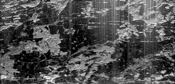
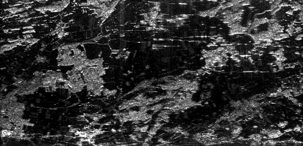
Figure 5 shows a P-Band image in the vicinity of Weilheim, Germany, which is severely degraded by RF interference. The image was generated by the experimental airborne SAR system E-SAR of the DLR, and the raw data was supplied to the authors by the DLR, Oberpfaffenhofen, Germany. The RF interference in the image is clearly visible as bright lines in the range direction. 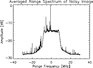The interference is more dominant at the far range due to sensitivity time control (STC). To obtain an estimate of the number of interfering sources, 100 range spectra were averaged. Since the interference remains relatively constant across a number of range lines, averaging a number of spectra enhances the visibility of the interference.

Figure 3: Averaged Range Spectrum of Noisy Image

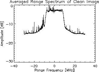
Figure 4: Averaged Range Spectrum of Cleaned Image

From Figure 3 one can see that there is a large interference spike near the origin, and about 15 smaller spikes on either side of the origin. After the image had been cleaned with a 512-tap adaptive filter, the same 100 range spectra were averaged, yielding the result shown in Figure 4. The large interference spike has been reduced by about 12dB, which is a significant improvement. However smaller interference spikes are still visible.

Figure 6 displays the cleaned P-Band image, which is definitely a vast improvement. Some features that were hidden by the interference have become visible, although sidelobes of bright targets have also become more pronounced. Future work will concentrate on reducing these sidelobes.

Figure 5: P-Band image in the vicinity of Weilheim, Germany, degraded by RF interference. The flight path is along the horizontal axis, with near range towards the bottom of the image. The raw data was supplied by the DLR, Oberpfaffenhofen, Germany.

Figure 6: The same image after applying the LMS adaptive filter to cancel the interference.

7 Conclusions

This paper has looked at a number of techniques that have been implemented to suppress RF interference, but only the LMS adaptive filter has been implemented and studied in detail, partly because of its ease of implementation, and partly because of its favourable review in the literature.

It has been found that the adaptive filter does significantly suppress RF interference, although sidelobes are enhanced. Future work will entail looking at further enhancements to the algorithm, like sidelobe reduction and computational efficiency.

Acknowledgments

Special thanks go to Stefan Buckreuss from the DLR for supplying the raw P-Band E-SAR data, and for his help with processing the data. The authors would also like to thank Jasper Horrell for his extensive help with processing the data, as well as Andrew Wilkinson for his stimulating discussions on the subject.

References

1: K. Abend and J. McCorkle, ``Radio and TV interference extraction for ultra-wideband radar,'' in Algorithms for Synthetic Aperture Radar Imagery II (D.A. Giglio, ed.), SPIE, Orlando, FL, vol. 2487, pp. 119-129, April 1995.
2: M. Braunstein, J. Ralston and D. Sparrow, ``Signal processing approaches to radio frequency interference (RFI) suppression,'' in Algorithms for Synthetic Aperture Radar Imagery (D.A. Giglio, ed.), SPIE, Orlando, FL, vol. 2230, pp. 190-208, April 1994.
3: S. Buckreuss, ``Filtering Interferences from P-Band SAR Data,'' Proc. European Conference on Synthetic Aperture Radar, EUSAR'98, Friedrichshafen, Germany, pp. 279-282, May 1998.
4: G. Cazzaniga and A.M. Guarnieri, ``Removing RF interferences from P-Band airplane SAR data,'' Proc. IEEE Geoscience Remote Sensing Symp., IGARSS'96, Lincoln, Nebraska, vol. 3, pp. 1845-1847, June 1996.
5: B.H. Ferrell, ``Interference Suppression in UHF Synthetic-Aperture Radar,'' in Algorithms for Synthetic Aperture Radar Imagery II (D.A. Giglio, ed.), SPIE, Orlando, FL, vol. 2487, pp. 96-106, April 1995.
6: J.R. Glover, Jr., ``Adaptive Noise Cancelling Applied to Sinusoidal Interferences,'' IEEE Transactions on Acoustics, Speech, and Signal Processing, vol. ASSP-25, no. 6, pp. 484-491, December 1977.
7: A. Golden, Jr., S.A. Werness, M. Stuff, S. DeGraaf and R. Sullivan, ``Radio frequency interference removal in a VHF/UHF deramp SAR,'' in Algorithms for Synthetic Aperture Radar Imagery II (D.A. Giglio, ed.), SPIE, Orlando, FL, vol. 2487, pp. 84-95, April 1995.
8: S. Haykin, Adaptive Filter Theory, 2nd edition, Prentice-Hall, Englewood Cliffs, NJ, 1991.
9: T. Koutsoudis and L. Lovas, ``RF Interference Suppression in Ultra Wideband Radar Receivers,'' in Algorithms for Synthetic Aperture Radar Imagery II (D.A. Giglio, ed.), SPIE, Orlando, FL, vol. 2487, pp. 107-118, April 1995.
10: C.T.C. Le, S. Hensley and E. Chapin, ``Adaptive Filtering of RFI in Wideband SAR Signals,'' 7th Annual JPL AirSAR Workshop, Pasadena, California, January 1997.
11: J. Li and P. Stoica, ``Adaptive Filtering Approach to Spectral Estimation and SAR Imaging,'' in Algorithms for Synthetic Aperture Radar Imagery II (D.A. Giglio, ed.), SPIE, Orlando, FL, vol. 2487, pp. 153-164, April 1995.
12: S.L. Marple, Jr., Digital Spectral Analysis, Prentice-Hall, Englewood Cliffs, NJ, 1987.
13: T. Miller, J. McCorkle and L. Potter, ``Near-least-squares radio frequency interference suppression,'' in Algorithms for Synthetic Aperture Radar Imagery II (D.A. Giglio, ed.), SPIE, Orlando, FL, vol. 2487, pp. 72-83, April 1995.
14: J.M. Ralston, J.F. Heagy and R.J. Sullivan, ``Environmental Noise Effects on VHF/UHF UWB SAR,'' Proc. European Conference on Synthetic Aperture Radar, EUSAR'98, Friedrichshafen, Germany, pp. 141-144, May 1998.
15: B. Widrow and J. McCool, ``The Complex LMS Algorithm,'' Proc. Letters of the IEEE, pp. 719-720, April 1975.
16: B. Widrow, J.R. Glover, Jr., J.M. McCool, J. Kaunitz, C.S. Williams, R.H. Hearn, J.R. Zeidler, E. Dong, Jr., and R.C. Goodlin, ``Adaptive Noise Cancelling: Principles and Applications,'' Proc. IEEE, vol. 63, no. 12, pp. 1692-1716, December 1975.
17: B. Widrow and S.D. Stearns, Adaptive Signal Processing, Prentice-Hall, Englewood Cliffs, NJ, 1985.; Return to Richard Lord's Homepage.